A few very simple notes on Quantum Computing.

Version : 1.1
Date : 10/05/2012
By : Albert van der Sel
For who : For anyone who likes a very simple introduction in Quantum Computing. Hopefully, it's any good.
Status: Still busy on it it ...

Quantum Computing (QC) is related to "Quantum Information Theory", in which the latter is a more generalized formulation, while
"Quantum Computing" is more oriented on research, and technical implementations of, suitable quantum states
which can be used for processing.

First of all, please don't get the wrong idea about this note. It's not about "Information Theory" at all.
It's only a very limited survey of Quantum Computing, in very general terms.

Quantum computing is not the usual trend we all know so well, namely the speeding up performance, and scaling down sizes,
of the computer hardware. No.., QC is really something fundamentally different. And this note is a very simple introduction
on this amazing science.

Chapter 1. Introduction.

1.1 Conventional computing.

When you take a look at the "fundamental" hardware architecture of "Conventional computers", we can observe many things,
but I would like you to focus on this fact only:
Buffers and Registers in a computer, are all over the place. RAM Memory is a serie of memorycells.
They all can hold "bits", which usually are Voltages (like some "+ Voltage" as a "1", and "0 Voltage" as a "0").

Now the essential thing of conventional computing, is this:

At any one time, the state of registers, or memory cells etc.. is fixed, or determined..
Ofcourse, the contens of, for example, a Register (or buffer or whatever part) can change very quickly, but at a certain time,
it just contains a series of fixed bits, like for example "0110111100110101".
At a certain point in time, it's completely determined.
So, if we take a "photo" or "screenshot" so to speak, we see a "fixed or determined state".

Any cell of whatever "memory" (register, RAM memory etc...) will hold only one of two values: a "1" or "0".
Any array of those cells, will hold just a fixed set of bits.

Ofcourse, if we would follow the state of registers for a duration of 1 second or so, we would go crazy: the state
would change tremendously fast.
Because computers are so fast these days, a new set of (say 32) bits is loaded, then a new one etc.. at a rapid pace.
But that's not the point. The point is: when loaded, it's fixed (determined), albeit maybe for a short time.

All this probably will not amaze you. In this sense, a conventional computers is pretty "exact". Suppose you have a chip, it
typically it will have a number of "inputlines" and "outputlines". A certain discrete set of input bits on the inputlines,
will produce a determined, exact, set of bits on the outputs.

Note 1:

I "over-idealized" matters a bit, because if you take a deeper look on what's going on in, say, a chip,
it's all solid-state physics, with quantum effects "all over the place".
While that is true, it does not "harm" the key point presented above.
I could, in principle, replace all electronics with just mechanical equivalents, like having a chip simulated by a sheet,
where all registers and buffers are represented by series of holes which hold (or doesn't hold) billiard balls.
Then, just by shufling around the balls through the various registers, I can simulate all logical AND, OR and other operations.

1.2 Quantum states & Superpositions.

Ofcourse, Quantum Mechanics (QM) is not a very trivial Theory. But the following key notions are not too hard to understand.

Let's first spend a few words on "Superposition". Superpositions can be found "everywhere", not only in QM.
For example, let us take a look a some basic mathematics:

Example 1:
Maybe you know that many functions can be written as the superposition of (infinitely) many sinusoids (Fourier analysis).

Example 2:
As another mathematical example, supose the functions f₁, f₂, and f₃ are solutions of a linear equation, then for example φ = c₁ f₁ + c₂ f₂ + c₃ f₃ is a solution too.

Example 3:
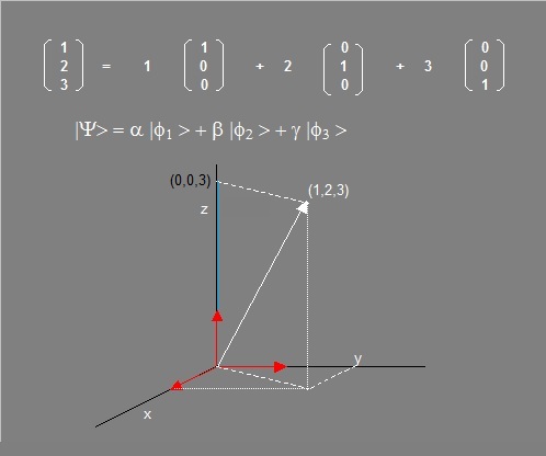
As yet another example: the vector (1,4,3) can be written as "1 x (1,0,0) + 4 x (0,1,0) + 3 x (0,0,1)"
where the (ortogonal) eigenvectors (1,0,0), (0,1,0), (0,0,1) are superimposed (or simply added) to form (1,4,3).

Let's return to physics. Even in classical physics, superposition is common business. Waves can superimpose (interfere)
Or, if we consider 3 charged particles is some region, the Electric field at some point is the superposition of all 3 individual fields
of those 3 particles.Indeed, we can go on and on in providing examples...

In QM, when finding the probability of some property (observable), it "works" the same way, although it is a bit "special".
Suppose we have a quantum system, for example, some sort of particle. Suppose further, for some observable property,
of that particle, that this property when measured can have either of two "values", or "states", namely |0> and |1>.

For now, don't worry about how we write stuff down, like |Ψ > or (0,0,1) etc.., it`s all just different ways to denote vectors.

The property we are talking about, could for example be some sort of angular momentum, that could have those values,
when we would measure it according to some direction.
Now, before we would actually measure that property, the system really is in a superposition of |0> and |1> at the same time,
like in the following equation:

Ψ = a|0> + b|1>

Usually, people say that the system is represented by the "wave function" ot "state vector" Ψ
The coefficients a and b, express the "probability" of obtaining the result |0>, or the result |1>, respectively.
Since the sum of the probabilities should be "1",it follows that |a|²+|b|²=1.

Maybe youre a bit puzzled now. Then you are not alone! Even the physicist that shaped QM, had a hard time, and even today
several interpretations exists. The problem is: the system is a combination of |0> and |1>, but when measured,
it collapses, or decoheres, into either |0> or |1>, with certain probabilities.

Note 2:

In general, a system can be in a superpostion of "eigenstates" (or eigenfunctions, just similar to the
eigenvectors of example 2 above).
When a measurement is done, it's actually a "perturbative" measurement. The QM "Decoherence Theory" might provide for
the best interpretation for the collapse of the wave function.
When the system "comes closer" to the measuring device (or just the environment), the system entangles with the device,
thereby forcing the "sort of" fitting eigenfunctions to be einselected (that is: selected).
Some people would say that the system decoheres into a particular eigenvalue.

As a weak analogy: if you throw a cake to a sharp metal grid, the environment (the grid) selects certain "aspects"
of the cake. If you used another orientation of such a grid, in principle, other results could have been obtained.
Ok, the analogy is not so terribly good, but hopefully you get the picture.
A point seems to be: In certain cases, if you want information (you measure), you destroy other information.

Note 3:

If you want, its perfectly "legal" to compare the state vector Ψ = a|0> + b|1> to a superposition of ordinary vectors,
like shown in the figure below.

Fig. 1: comparison of the statevector Ψ to ordinary vectors .

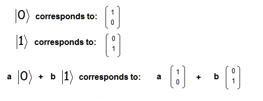
Actually, Ψ = a|0> + b|1> is a "qubit" or a Quantum bit. The special thing about the Quantum bit is, that it is
a superposition of "|0>" and "|1>" at the same time! (unless it collapses, or decoheres, to a particular state).

Since the (probability) coefficients a,b have to meet the relation |a|²+|b|²=1 (because the total
probability must be "1"), they actually define a circle (or sphere), which often is called the "Bloch sphere".

1.3 Quantum Bits or "Qubits".

In section 1.2, we have seen the general equation of a qubit, or Quantum Bit, which exists in the
superposition of the states "|0>" and "|1>", simultaniously.

Wave function Qubit: Ψ = a|0> + b|1> (equation 1)

Now, those states can be interpreted as the bits "0" and "1". You don't believe that? Sure they can !
Even in the classical situation, you just need two different "states" that enables you to make a clear distinction
between the two, and next you only need to label them "0" and "1".

Up to this moment, we haven't discussed "true" Quantum Computing (QC) yet. That will be the subject of chapter 2.
But I am sure that you already know by now (or intuitively feel), that "qubits" are essential ingredients for QC.

More extended quantum systems are possible too, like a "two-qubit" system.
Although we havent seen "real" world qubits yet in this note, or extended versions thereof,
the general wave function equation of a "two-qubit" (non-entangled) system would be:

Wave function (non-entangled) Two-Qubit system: Ψ = a|00> + b|11> + c|01> + d|10>

Here, the system exists in the states |00>, |11>, |01> and |01>, at the same time (simultaneously).

Especially, the more qubits you have to your disposal, the better your Quantum Computer will be.
As you might already have expected, since we have qubits, we could arrange a number of entangled qubits together
which then forms a "qubit register"
.

1.4 Multiple Valued quantum logic and "Qutrits".

One active field of research is using multiplevalued quantum logic, where more than two quantum basis states are used.
You know that the "ordinary" Qubit uses the states |0> and |1>. Could that even be enlarged?

New research is also focusing on using more than two base states, like for instance |0> and |1> and |2> as base states.
This then, might be called "ternary" quantum logic, where such a qubit then should be called a qutrit.
Such an undisturbed qutrit whould then be in a superpostion of those three states simultaneously, as in:

Ψ = a|0> + b|1> + c|2>

As we will see later on, most physical systems "naturaly" uses 2 base states like for example the spin of a electron, where the base states
be "up" or "down" with respect to a certain direction. Thats why much research was done by using Qubits.
However, it is obvious that the computational advantages of qutrits are higher compared to the ordinary qubits.

Some physicists already make a distinction in two types of QC, namely:

- Binary QC, using qubits.
- Multiple Value QC, using qutrits (and even entities with more than 3 base states)

For the time being however, we will concentrate on the more general aspects of QC, and much QC theory just simply
focuses in using and implementing qubits.

1.5 Entangled qubits.

Quantum entanglement is also a form of quantum superposition. It is this:, if two (or more) particles are entangled,
one particle cannot be fully described without considering the other particle.
They will stay in a "quantum superposition" and share a single quantum state, until a measurement is made

When a measurement is made on one member of such a pair, and a definite value, for example "value X", is found,
the other member of this entangled pair will always be found to have taken the correlated value "value Y".

Actually, entanglement is really cool (and absolutely mindboggling at times).

Why don't we have FUN for a moment, take a closer look at a famous example?

Here is the example: A pair of spin-1/2 particles (particle A and particle B) can be combined to form three states
of total spin 1 (called the triplet), or a state of spin 0 (which is called the singlet).
Let's take a look a the spin 0 case.

The equation for this state can be written as:

wave function for this entangled system: Ψa,b=1 / √ 2 ( |↑ ↓> + |↓ ↑> ) (equation 2)

Take a good look at equation 2. Now notice this: It's a quantum superposition of two states ↑ ↓ and ↓ ↑,
which we might call "state 1" and "state 2". In such a state as for example | ↑ ↓ >
we see particle A as ↑ and particle B as ↓

In state 1, Particle A has spin along +z and particle B has spin along -z.

In state 2, Particle A has spin along -z and particle B has spin along +z.

(here in this example, we look with respect to the z direction; but any other direction could have been choosen)

Now suppose the particles are moving in opposite directions.

Alice has placed a detector where particle A will fly by, and Bob did the same at where particle B goes to.
Alice now measures the spin along the z-axis. She can obtain one of two possible outcomes: +z or -z.

Suppose she gets +z. According to what we know of the collapse of the wave function, the quantum state of the system
will collapse into state 1.
Thus Bob then will measure -z. Similarly, if Alice measures -z, Bob for sure will get +z.
No matter what the distance between Alice and Bob is.

Isn't that amazing? If Alice gets +z, Bob gets -z, and the other way around. How do both particles know that?
I mean: the entangled system is in a superposition of |↑ ↓> and |↓ ↑>.
Especially when the distance between particle A and particle B is large, it's quite puzzling.
However, most physicist don't believe that a superluminal (faster than light) signalling operation is at work here.
But what is it then?

First I have to admit that in the example above, I oversimplified matters. In experiments, in fact statistical results
are obtained, using many entangled particle systems. Due to various reasons, not only the spin along z is measured, but also along
the x (or y) direction. Finally, the results are tested agains te socalled "Bell" (or derived) inequalities.
But.. currently, all results seem to sustain the conclusion of the example presented above.

Many "suggestions" have been forwarden, like "hidden variables" (which we don't know of yet), which works in such way
so that from the start of entanglement, a sort of hidden "contract" can explain the oserved effects.
But many other "explanations" go around too, like Multiple Universes (MWI), or some still do believe that a "spooky action"
that exceeds the speed of light is at work, or that our interpretation of space-time isn't correct etc.. etc..
However, many physicists say that the observed results happen with "probabilities" (see note below) and this type of correlation
does not automatically imply communication.
Indeed, most physicist accept that non-locality effects of this sort, is simply "non-signalling".

However facinating it is, we better not let it be part of a simple note of Quantum Computing.
(But if your interested, search the net on EPR, hidden variables, spooky action at a distance , Bell inequalities)

Back to our QC discussion: the following is very important!

"Equation 2" also is a superposition of two states, just like "equation 1" from section 1.3 is.
In terms of superpostions of "0" and "1", it is quite the same, so here we have an qubit too, albeit an entangled one.

One reason to use entangled systems, is that they are somewhat more robust for decoherence.
Another reason can be the initial "lining up" (interaction), and associated "loading" of an algolrithm.

In the text above, we just looked at a system of a 2 qubit system. In this case, here only 2 types of entanglement are possible, namely
or they are seperated or they are entangled.
It's probably too much overstated if we say that an entangled 2 qubit system is understood. But at least we can "write" down
the equation in ket or vector notation.

But describing a system of three (or more) entangled qubits, is by no means a trivial matter !.
It's even fair to say that an N entangled qubit system (say N>6) is not even fully explored (maybe you are a bit amazed by that).
Things like "pairwise" entanglement pops up, and many other stuff needs to be taken into consideration.
It looks like it's all so simple, but it's not.
And ofcourse: what property or observable you are looking at? Spins or another propery? This is important too.

To get an impression:

Three qubits can be entangled in fundamentally different ways. For certain systems, you might find the states:

|GHZ> = ( |000 >+|111 > ) /√2 (equation 3)

|W> = ( |001 >+|010 >+|100 > ) /√3 (equation 4)

Which indeed are quitedifferent.

Anyway, by now, we have some sort of a "reasonable" impression about entanglement.

1.6 Some implementations of qubits.

When fabricating qubits, physicist have a number of considerations to do:

The threat of Decoherence:

The scientist who want to realize QC, usually struggle with "decoherence" (see section 1.2), which always threatens a Qubit
to "collapse" to a single state. So, how do they control the qubits? Or, the question rephrased in other words:
What implementations are out there in the real world? Indeed, in the following we will "nimbly" touch a few examples
and milestones.
As we already have seen in section 1.5, entanglement often provides for "tougher" qubits or n-qubits.
But, if a system is too strongly entangled, it might even overshoot the practicle usage for qubits.

Also, the more qubits are involved, the more the "danger" exists that quantum information will "disperse" into the environment,
and that would destroy the computation.

What can be a Qubit?:

Actually, the whole question boils down to: How To Construct Qubits in physical systems?

Researchers might consider any system or entity that could potentionally work as a qubit, like for example molecules, atoms, ions, photons,
electrons, or any other particle or system. Thus, In principle, any system having an observable quantity which has at least two
discrete eigenvalues, could be a "candidate" for a qubit. Again, unmeasured, the system would be in a superposition of those states.

Ofcourse, a need for "control" exists too.
You might for example say that a 1/2 spin particle, or two entangled particles in the singlet state, could in principle
act like a qubit, but don't you need to "store" it somewhere too?
Also, any influence that decoheres the system, like "noise", or any influence from the "environment", should be below certain tresholds.

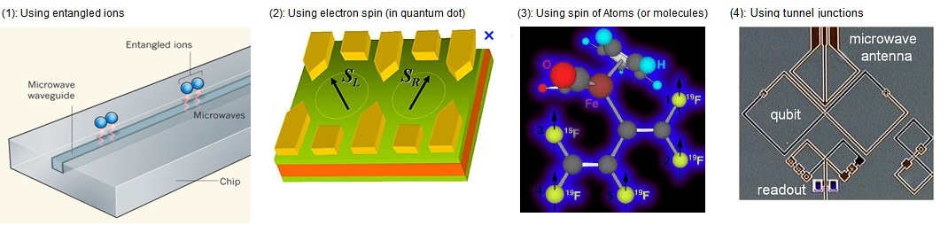
Some examples:

⇒ One example of a qubit, or a two-state quantum system, is the polarization of a single photon,
where we refer to the two states of vertical polarization and horizontal polarization. But, a photon travels, so here
we have the difficulty of "storage", unless the propagation in fiber (or other way to "trap" it) would be no problem.

⇒ Another example could be a 1/2 spin particle, like an electron. Here too, the spin with respect to a certain direction
is discrete, and is often notated as |0> and |1>, or as |↑> and |↓>.
But as we have seen in the former section, two of those particles can form an entangled state, which often has advantages above single particles.
But ever so often, especially if implemented in solid state environments, single electrons are also often used.

But it is by no means limited to the use of electrons. Also any system with a result spin, like a nucleus, could be used too.
The advantage of using the spins of nuclea, is that the qubits are naturaly "trapped" within a molecule.

⇒ Following the former example, physicists have indeed used nuclea of larger molecules, in a liquid solution,
as an implementation of an n-qubit (like 5 or 8 qubits).

⇒ Using electron spins isolated in socalled "quantum dots", placed in sort of a semi-conductor like "chip",
seems as a very practical solution for implementing qubits.
Then, often electro-magnetic fields are used to control the qubits. This is very effective, since we need something
like a "gate" too for implementing computations.

⇒ As the last example, "tunneling junctions" in semiconductors have proven to be very promising too.
Here, superconducting "islands" are connected by tunnel junctions, which provides for the behaviour of true qubits.

Fig. 2: Some examples of qubits.

Some important and recent investigations use excited electrons, which leave a "hole" in some sort of cristalline material.
This "hole" much resembles the electron's anti-particle, which gives rise to an (almost?) "Majorana" like particle.
Indeed, recent results seems to indicate that those discoveries might have large implications for QC in the foreseeable future,
because these Majorana particles seems to be very robust in the environment, making them very good candidates
for long lasting qubits.

Now, it would be ideal, if the qubit(s) and the gate are sort of integrated. For example, in a semiconductor implementation,
where for example an electron is (sort of) captured, or an electron and a nucleus are present (in either case using the
the familiar spin), several microscopic "wires" in vincinity, can be used for the inputs/outputs/controls of the gate.
The wires here, are usually not physical wires: it can be a EM field (a photon), a property of a particle etc..

From what you can find on the Internet, some sites or manufacturers make truly astonishing claims!
Sometimes you might wonder whether they are really talking about QC at all.
Just fort getting an impression, if a Lab knows how to fabricate a 14 qubit system, then thats really quite some achievement.

1.7 Gates

Classical Gates:

Mind you, the following is NOT about quantum gates and QC, but instead it`s about conventional computing.

With respect to the physical implementation of conventional gates: just open any conventional computer, or take a
a look at any card or board: it`s just full of "chips". Indeed, its all about integrated circuits.
All those circuits are "arranged" in such a way, that a large number of logical Boolean gates are implemented
which do all sorts of operations on (true) classical (static) bits.

Now, the classical logical gates (like "AND", "XOR" and all others, except the NOT gate), are not reversible .
Why would that be important? This will be answered in a minute. Let`s first take a look at typical classical gate,
as is shown below in figure 3.

Fig. 3: An example of a classical (conventional) logical gate. In this example, the AND gate.

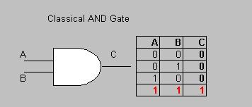
Here you see the input ports A and B, and the output C. Only if A and B are both "1", the output is "1" too,
otherwise, in all cases, the output C will be "0". You can see in upper table all possible combinations of inputs A and B,
and what the result C will be. So, for A and B in (0,0), (0,1), (1,0), the output C will be "0".
So, given C=0, we simply cannot know what the inputs were. There are multiple combinations for A and B
that will result in C=0. So, this classical gate is not reversible.

Note 4:

It`s really proven that even classical gates can be made "reversible", for example, using additional junk-control lines.
Also, irreversible classical gates can become reversible gates where we hardwire some inputs and throw away some outputs.
Note that there are very interresting discussions about the degree of entropy of reversible/irreversible circuits.
For this ultra-super-hyper simple note, I will just leave that out.

Quantum Gates:

For the physical implementation, the qubit(s) and the neccessary controls are too often "integrated". As an example
of a semiconductor implementation, take a look at example 4 in figure 2.
Indeed, such a setup is quite convienient, but certainly not a requierement. So, suppose you just have a bunch of molecules
in some liquid, which just happens to be good longlasting qubits, and using EM radiation for control and read-out,
that would be great too.

The follwing is quite important for understanding Quantum Gates.

When the process of computation is going on, the superposition at the qubits should not be disturbed.
You know that if we do something that resembles a measurement, the system collapses to an eigenvalue.

So, we may treat the system as a normal time evolution of just any other undisturbed (nonmeasured) quantum system.
Dont say "whats this?" for the following right away, since it all can be explained:

The evolution, or transformation, the system undergoes can be expressed by

ih ∂ |Ψ>/ ∂ t = Η |Ψ> (equation 5)

The "ih" can be considered to be just a constant, so we dont worry about it. What the equation says is no more than "the change of the system in time"
(notated by ∂ |Ψ>/ ∂ t), is the effect of the Hamiltionian "Η" which just stands for all forces and fields operating on the system.
That makes sense, doesn't it? A system changes in time due to the forces or fields acting on it.

You have seen before (like e.g.|Ψ> = a|0> + b|1>) that quantum systems can be interpreted as a "state vector", and you can
decompose such a system as a superposition (or addition) of eigenvectors (base vectors).
From that viewpoint, it's really a small step to matrix calculus. Maybe you already know (from no more than highschool mathematics)
that operations on vectors is done by operators represented by matrices.
Don't forget that |Ψ> is actually a vector (sort of), and that for our qubit systems, we may rewrite equation 3 as:

|Ψ(t) > = U |Ψ(0) > (equation 6)
'
Where "U" is some (unitary) matrix (!). We will not bother ourselves too much on what exactly unitary means.

The essential thing here is:

do you agree (or do you find it acceptable) that our system, the qubit(s), will evolve
from some initial state |Ψ(0)> to a later state |Ψ(t)>, due to the "transformation" or "operator" U which can be
represented by a matrix?

If you do, an important step has been taken, since Quantum Gates are described, mathematically, by unitary matrices,
and their actions are always logically reversible.

Indeed, once you realize that our systems can be represented by vectors, the step to matrices is not so far away.

So, when studying articles on QC or Quantum Gates, besides logical diagrams or physical implementations, you should
expect to see the corresponding matrix which actually really defines the gate (!)
Indeed, no matter what (possibly horrible complex) logical diagram you will find in some article,
it's really the matrix that decribes the Quantum operation, or the Quantum Gate.

Note 5:

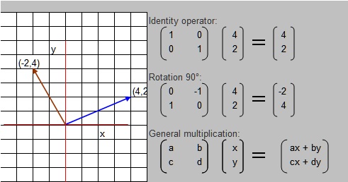
Just to illustrate this stuff a bit:
Below are a few basic examples on how to represent operations (on vectors) by matrices. Here, the examples are in R².
It is no more than a bit of highschool mathematics, but still it nicely illustrates the key points here.
For example, the vector (4,2) does not change at all by the "Identity" operator (which has all 0`s, except in the diagonal).
However, the vector (4,2) is mapped to (-2,4) by the matrix that represents a Rotation over 90 degrees.

Fig 4.

Chapter 2. Some basics of ket algebra.

In order to make sure we can get a basic understanding of quantum circuits and gates, we just need a tiny understanding
of ket algebra first. I first thought I could escape that, but I was somewhat naive, and now I concluded that it's
really not possible. But..., actually that's not so bad at all !
So, lets review a few basic facts of Ket algebra.

2.1 Analogy from regular vector calculus:

Let's start with a simple analogy from mathematics. Take a look at "ordinary" vectors in 3 Dimensional space.
For example, the vector V=(1,2,3) can be represented as

(1,2,3)=1x(1,0,0)+2x(0,1,0)+3x(0,0,1)

which is actually the addition (superposition) of the 3 base vectors (1,0,0), (0,1,0), and (0,0,1).
These base vectors have a "lenght" of "1", and are oriented, respectively, along the x, y, and z axis.
So, the are all perpendicular to each other, or in other words: they are orthogonal

In order to get (1,2,3), we need to add 1x(1,0,0)+2x(0,1,0)+3x(0,0,1)=(1,0,0)+(0,2,0)+(0,0,3)
Note that if we "project" V, for example, onto the z-axis, we get the "projection" (0,0,3)
It's the same as if we would say that we need to multiply the base vector (0,0,1) by 3, in order to get (0,0,3),
which is indeed that projection of V on the z-axis.

Note that in regular vector calculus, vectors are often denoted as row vectors or as columnvectors (as shown in the figure below).

Fig 5. Simple analogy using familiar vectors in 3 dimensionalspace (R³)

2.2 What is the "ket" representation of a quantum system?

With Ket algebra, the situation is not unlike to what we have seen above. An observable of a quantum system, can be described by a "Ket" vector,
denoted by |Ψ > in an n dimensional "space", which is often called "Hilbert" space.
Now, suppose that this observable can have a number of "n" values that it can attain (when measured), then we can write the ket as

|Ψ > = c₁|φ₁ >+ c₂|φ₂ >+...+ c_n|φ_n > = ∑ c_i |φ_i > (equation 7)

See? It just looks like a regular vector.
Here, we can view the state |Ψ > as being in a superposition of the basis states |φ₁ > + |φ₂ > ...
So, just as with "regular" vector calculus, if a basis is chosen for the Hilbert space of a system, then the ket can be expanded
as a linear combination of those basis elements (or basis states).

The coefficients c₁, c₂.... then corresponds to the probability of finding the observable in such a basis state.

If we return to our qubit system that was introduced in section 1.3, we saw that the basis states were |0> and |1>.
Yes, here we have only two basis states, which we could have denoted by |φ₁ > and |φ₂ >
But since it's often related to the spin of a system, which can be "up" or "down" with respect to a certain direction,
physicists usually write the states as |↑> and |↓> or as |0> and |1>. But that does not change anything fundamentally.

In superpostion (that is unmeasured), the qubit is in both states simultaneously, which we write as:

|Ψ > = a|0> + b|1>

Here too, the coefficients a and b, express the "probability" of obtaining the result |0>, or the result |1>, respectively.
Since the sum of the probabilities should be "1",it follows that |a|²+|b|²=1.

The basis kets |φ_i are often called "eigenstates", where the corresponding coefficient is called the "eigenvalue",
which corresponds to the probability of finding the Observable to have that particular value

Maybe you buy it that a quantum state can be expressed as a Ket vector as we just did. But why the coefficients corresponds
to the probabilities of finding a certain eigenvalue, that might be tougher. There are just many interpretations for this problem.
The Copenhagen interpretation speaks of the "collapse of the state vector" if a measurement is done, which can be viewed as
a projection of the Ket onto just one of the basis states.

A more modern interpretation says that the state in superposition, when measured, decoheres into states that are
selected (so to speak) by the environment or the measuring apparatus.
Don't forget that a "measurement" on a microscopic system, might be viewed as very perturbative: it has a really strong effect.

In section 2.3, I will come up with a reasonable interpretation why such a coefficient it is connected to the probability.

Note: we assume that we deal with normalized systems, so that the sum of the squares of the coefficients, equals "1".

2.3 Inner product of Kets, or the Projection:

Maybe you know of the "inner product" of two regular vectors in, say, two dimensional space, (or three dimensional space
or n dimensional space for that matter): the rules are always the same . The inner product returns a number.
So, suppose we take a look at two vectors in the plane (two dimensional space), say v and w.
Suppose that v=(v₁,v₂) and w=(w₁,w₂), here expressed as row vectors.
Then the inner product v . w is defined as:

v . w=v₁.w₁+v₂.w₂
So if for example v=(2,3) and w=(1,2), the inner product is: 2x1 + 3x2 = 8

A special case arises, if we calculate the inner product of a vector, say (2,3) with one of the "basis vectors",like (0,1),
which is the unit(basis) vector along the y axis.

that will be: 2x0+3x1=3

Which is exactly the length of the "projection" of (2,3) onto the y-axis.
Note that the inner products of the basis vectors are either 0 or 1: for example:

(1,0) . (0,1) = 0 + 0 = 0
(1,0) . (1,0) = 1 + 0 = 1

For kets, a similar product is defined. Before we go to the conjugate partner of a ket, called the "bra", I will be a bit naughty,
and explain the ket "inner product" in the following way. Instead of explaing "bra's" right now, I will just make a parallel
with the ordinary inner product of vectors.

The inner product of the kets |Ψ> and |Φ> is notated as:

< Φ| Ψ >

Actually, its quite similar to "ordinairy" vectors. Let's immediately g to an interesting special case.
Let's see what the inner product is of an arbitray ket and one of it's basis states (one of it's eigenvectors), say |φ₂ > :

<φ₂ | Ψ > = <φ₂| ( c₁|φ₁ >+ c₂|φ₂ >+c₃|φ₃ >+...+ c_n|φ_n >) =

c₁<φ₂;|φ₁ >+ c₂<φ₂|φ₂ >+c₂<φ₂|φ₃ >...+ c_n<φ₂|φ_n > = c₂ (equation 8)

It's indeed "c₂", since terms like <φ₂|φ₃ > are 0, since these basis vectors are orthogonal,
and only <φ₂|φ₂ > is 1 in equation 8.
Indeed, <φ_i|φ_j > =0, for all i,j unless i=j.

You see? The "projection" or "collaps" of | Ψ > on the eigen (basis) state |φ₂ > is associated to the number c₂.

However, |φ₂ > is a normalized basis ket with a length of "1", so there is no coefficient for |φ₂ >
to "worry" about.

When you take the inner product of two vectors in "Real" euclidean space, then we are dealing with
coefficients which are all socalled "real" numbers (like 1,5,-20,1.77, √, 0.99887 etc..).
So, suppose we have the vectors v=(1,1,1) and w=(-1,3,2), then v.w=-1+3+2=4, which is again a real number.

But kets in general have coefficients from the complex number "set". The inner product produces a complex number.
If you expand < Φ| Ψ > in their basis kets, then we need to take the complex conjugate of the coefficients
of the ket (bra) "of the left side", meaning:

if | Φ_a > = a₁|φ₁ > + a₂|φ₂ + a₃|φ₃
and
if | Φ_b > = b₁|φ₁ > + b₂|φ₂ + b₃|φ₃

then

<Φ_a | Φ_b > = a^*₁b₁ + a^*₂b₂ + a^*₃b₃ = ∑a^*_jb_j (equation 9)

Note:

You might wonder: why with "real number" vectors (real coefficients) we just do v₁.w₁+v₂w₂+..., while with vectors in Complex space,
we need to use v^*₁.w₁+v^*₂w₂+... where for example v^*₁ is the complex conjugate of v₁?
This is so, because mathematically it is (sort of) demanded that also in Complex vectorspace, it must hold that
v.w = (w.v)^*, which is the complex requirement of the "real" counterpart of the ordinary requirement that a.b = b.a where a and b are vectors in real euclidean space.

In figure 6 below, we repeated the discussion for our well-known qubit. As you know, the ket |Ψ > = a|0> + b|1>
can be expanded on |0> and |1> as it's the basis states. Since |0> and |1> are orthogonal and normalized, we have for example <1|0>=0 and <1|1>=1.

Fig 6. Projection of the qubit on one of it's basis states.

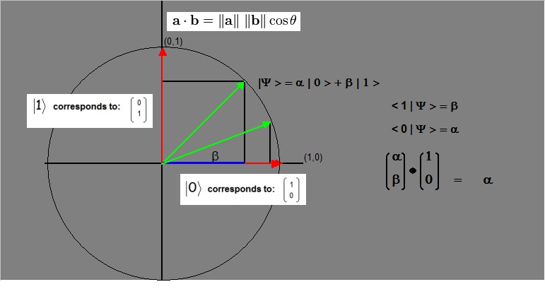
If we now take the inner product <1|Ψ > = a <1|0> + b <1|1> = 0 + b =b

You really may interpret the inner product of |Ψ > with one of the basis states, as the "projection" or "collapse"
of |Ψ > on that particular basis state. In the figure, this is illustrated by the blue line.
The true probability for this collapse onto |1> is actually:

| <1|Ψ > |² = |b|²

Indeed, we already have seen the sum of all probabilities before. Its |a|²+|b|²=1.

Above we said that for ortonormal basis states, we have <φ_i|φ_j > =0, for all i,j unless i=j.
This is also often expressed as <φ_i|φ_j > = δ_ij
where δ_ij = 0 for all i and j, unless i=j.

A few words on the "bra" < Φ|

Maybe I should have started the discussion about the inner product, by introducing bra vectors. Bra vectors (or bra states)
are notated like < Φ|

While Kets and basis kets are more easily associated with quantum states, a bra is not so easy to associate with a quantum state.
But the concept is quite important in calculations and derivations. So, what is it?

First of all, it's most important to understand kets and basis states as we already have seen above.

It is only just that bra's often are found in other articles, that we must introduce them here too.

Here are several interpretations:

(1):
For the inner product of the kets |A> and |B>, we notate it as < A | B >, and in this notation we call < A| the Bra, and |B > the Ket.
Most often it's physically interpreted as the chance of the projection of |B> onto |A>, as we already have seen happening above.
Indeed, the inner product is a number, and not a vector.

To be more exact: the probability of the state | ψ > jumping (collapsing) to the eigenstate | φ >is denoted in bra-ket notation by:

|< φ| ψ >|² (equation 10)

just as we have seen with the qubit, jumping to eigenstate |1>, which has the probability | <1|Ψ > |² = |b|²

(2):
The following interpretation actually "resembles" (1) a lot:
The bra < A | can be interpreted as a linear functional on a ket, that is, it's an operator that takes as input a ket,
and outputs a (complex) number. This is true. Because it's just the inner product which produces a number. For example, take a look at equation 8,
or any other inner product equation we have seen above.

(3):
Formally, a Bra is introduced as the "complex conjugate" of a Ket. What is this supposed to mean? Good question.
We haven't spend much words on the coefficients of a Ket in the expansion of that Ket in basis vectors.
Those coefficients just seem to be numbers.
They are indeed numbers, but actually socalled "complex numbers", which can have a "complex conjugate" partner number.
It's a sort of mirroring of the original complex number.

Furthermore, any Ket has an associated Bra, which is it's complex conjugate, that is:
Each ket |Ψ > is uniquely associated with a so-called bra, denoted as < Ψ|, for which the following holds:

If we have the Ket |Ψ > as:

|Ψ > = c₁|φ₁ >+ c₂|φ₂ >+...

then the uniquely associated Bra is:

< Ψ| = c₁^* <φ₁| + c₂^* <φ₂| + ...

where for example the c₁^* number, is the complex conjugate of the c₁ number.

(4):
If a Ket |Ψ > is known, the corresponding bra-vector < Ψ| describes the same state, i.e. it does not provide any other
information about the system and is only used for mathematical convenience, like in describing and notating operators.

Actually, interpretations (1) and (2) (who are almost identical), and (4), are quite "likeable", because the bra can be viewed as just an "operator".

2.4 Combined states or product states, and the "outer product":

Contrary to an entangled state of, say, two particles, a product state correspond to the situation in which each particle
is prepared independently, and can be measured independently.

Somehow, the ket's "overlap", and if we expand both ket's in their basis states, we can clearly see the endresult.

Mathematically, we need to sort of "multiply" both kets, which is called the "outer product", which is know in vector calculus too.
The result is that a new ket is constructed, again as a lineair combination of basis kets. A sort of "joint state".

Supose we have the kets |φ > and |ψ >

We have to take care here, because actually two types of outer products can be used, namely:

|ψ ><φ| which produces a matrix, or an operator.

|ψ > ⊗ |φ > which produces the product state, which is the, say, combined state (new ket).

We will first take a look at the normal product state. A bit later we will see how Matrices are produced (or notated in ket language)

Suppose we have two qubits like:

|φ₁ > = a|0> + b|1>

|φ₂ > = c|0> + d|1>

then:

|Ψ> = |φ₁ > ⊗ |φ₂ > = ac|00> + bd|11> + ad|01> + bc|10> (equation 11)

This joint state is not entangled, and is just a way to denote that joint state of the qubits.

|ψ > ⊗ |φ > is also notated in many articles as simply |ψ>|φ> or as | ψφ>

2.5 Operators, matrices, and "outer product" :

Chapter 3. Quantum circuits and computations.

Not ready yet.